Technote: Inventor Quick Tip

When working in Inventor you can access a list of Recent files by clicking the right mouse button on the Taskbar icon.
This also works for most programs with an icon on the Taskbar like Microsoft Excel, Notepad etc.
Technote: Inventor Quick Tip
When working in Inventor you can access a list of Recent files by clicking the right mouse button on the Taskbar icon.
This also works for most programs with an icon on the Taskbar like Microsoft Excel, Notepad etc.
Technote: Positioning Holes in Complex Surfaces
When detailing the skin panels for aircraft it can be quite daunting trying to locate a series of holes accurately at a specified distance from the edge of the panel. Typically fillets to wings and horizontal stabilizers and transition pieces to vertical stabilizers are all complex surfaces.


In this example, we need a series of holes located 17.5 mm from the top and bottom edges. As you can see the surface at the top and the flange angle at the base varies.
The location of the first hole, top and bottom, is aligned vertically so we first create a workplane to determine the horizontal position of the first hole. Ultimately we will use a 3d intersection curve for the centre line of the holes which must first be determined by sweeping a circle profile sketch along the edge as a surface with the radius set to the required edge distance. Using a circular profile for the sweep ensures that any intersection point on the surface will be at the specified edge distance.


This swept surface is then trimmed to the first work plane to define the start point of the 3d surface intersection curve as shown.


The resulting 3d spline represents the line of the hole centres at 17.5mm from any point along the edge of the fillet.
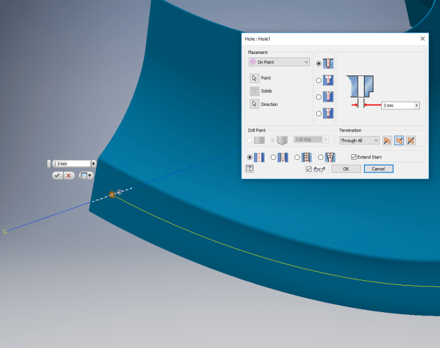
We then apply a point and an axis (perpendicular to the surface) at this point to determine the hole direction. I suspect because it is not a regular surface the hole feature will not allow me to select the surface for direction. Use “Extend Start” when creating hole.
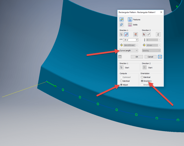
To pattern the hole along the spline and be perpendicular to the surface create the array as shown below. Be sure to select the extended options for “Direction 1” and “Adjust”.
Do the same for the top array of holes, resulting in 2 sets of holes aligned with the surface at 17.5 mm from the edge.

This works for the vast majority of riveted panel connections where locally there is a degreee of flatness between the matching parts. In instances, where there is extreme curvature of the connecting faces the radius of the extruded circle would have to be adjusted accordingly.
Grumman F6F Hellcat: Ordinates
I am without access to a Cad system for a few weeks so I decided to spend time reviewing my archive collection. Whilst looking through the many aircraft in the archives I came across some interesting information for the Grumman F6F Hellcat.

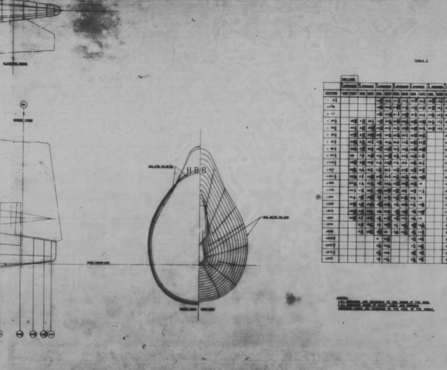
The archive consists of a substantial number of the Grumman drawings, varying in quality from very good to very poor, though I should clarify the latter relates to only a small number of drawings. This archive includes ordinate tables for the wings and fuselage so I figured it might be a worthwhile project to attempt to decipher and create a set of ordinate spreadsheets as I have done previously for the Mustang P-51.
Though I rather like this aircraft it was not a priority project on my to-do-list, but having spent today studying the Grumman drawings this could turn out to be a rather challenging project.
Fuselage Work in progress:

Update:
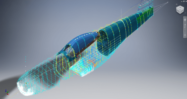
 I have managed to obtain a trial copy of the Inventor LT so I can now move ahead with this project. This first interpretation of the fuselage profiles is actually not bad at all. A few macro adjustments will be required to get the profiles correct, mainly due to the quality of the archive where roughly 10% of the values are very difficult to read.
Each point represents the ordinate of the longitudinal stringers which I will profile to assess the alignment and curvature as an aid to finalizing the frame ordinates. Perfecting the frame ordinates can become quite tricky at this stage, requiring constant referencing of the original drawings including the frame structures themselves which often provide additional information that can assist with this process.
NAA P-51D Mustang: Master Lines Plan
The P-51D project is progressing well with further developments on the fuselage frame profiles. I now have a comprehensive Master Lines Plan incorporating additional information obtained from mathematical analysis, drawings, reference documentation and geometric developments. I have updated and remodeled the underside Oil Cooler Air intakes, canopy, windshield, rear fuselage and fuselage tail-end. As part of the remodel the groups of ordinates for each frame for the Oil Radiator Duct, Coolant radiator Duct and Removable Scoop are now contained on their own respective work-planes. This will make it much easier to micro manage the final mold lines.
Fuselage Master Lines Plan (P-51D overlaid on P-51 B/C):

Test Lofts and developments:
Front Views (note the Canopy Profile update from the previous article):


A month ago I was not sure how much could be achieved given the limited amount of information at hand but with due diligence and detailed research, it is quite amazing what can be accomplished.
With this template, it is now technically possible to accurately develop a CAD model for the entire fuselage structure and mechanical components for the P-51D, which would be great; but I often wonder what the value of such an undertaking would achieve, other than being a darn interesting thing to do and a test of CAD modeling skills.
Having achieved this significant milestone the time is right to conclude the work on the Mustang P-51D and P-51 B/C projects. I may continue with the P-39 project but as always I am keen to explore the options for the more obscure extinct aircraft as described in Operation Ark.

If you are planning on developing your own Master Lines plan a good place to start would be with the 1000’s of ordinates points cataloged and recorded on the spreadsheets here: Mustang P-51B/C Ordinates which also includes the wing ordinates for the P-51D and vertical stabilizer.
NAA P-51D Mustang: Canopy
With the return to the P-51D project, I have been working on developing the fuselage and the canopy ordinates specific to the P-51D. Supporting information in this regard is hard to come by and we don’t have the luxury of tabulated ordinate values and fully detailed mold lines as we had with the P-51 B/C.
What we do have though is critical dimensions scattered amongst the 100s of drawings and documents that collectively help establish key datum points which in conjunction with conic geometric development appear to make this aspiration a feasible prospect. To give you some idea of progress this is a front view of the preliminary P-51D canopy model.
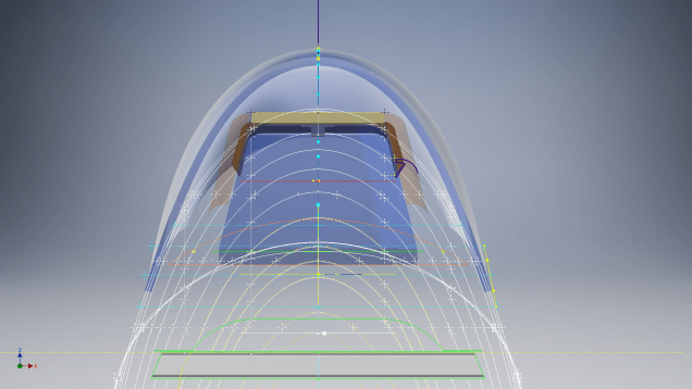
I still have the windshield model to develop in order to finalise the canopy design but I am pleased with achieving this amount of progress derived from many hours of research and some straightforward geometric developments. Notice in particular the accurate tangency alignment with the known frame mold lines, it is perfectly aligned. I appreciate that there are a few variations on the profile of the canopies that were made for the P-51; some more bulbous than others, but we first need to establish a baseline which is what we will have.
As a consequence of this activity, I have also managed to develop the rear fuselage profile ordinates for the P-51D. I am rather excited by this new development in conjunction with the completed wing ordinates and the more recent vertical stabiliser it may actually be possible to have a full ordinate set uniquely for the P-51D.
Update: Below is the finished baseline canopy model profile.
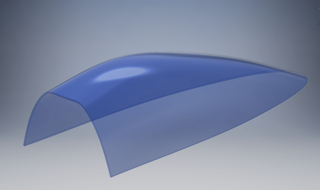
…and this is what it looks like to develop the canopy and windshield with limited known data…

Update: August 2018 “P-51D Bubble Canopy”


The real thing…this is a model derived from a ridiculously accurate laser scan point cloud of a P-51D Bubble Canopy.
NAA P-51 Mustang: Using Ordinate Data Spreadsheets
A question arose during a telecon today about using the Ordinate Spreadsheets for Cad and Modelling.
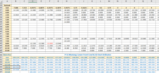
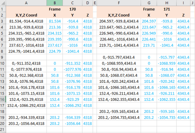
Typically for the fuselage and cowlings, the spreadsheets are set out as above. The top section replicates the layout of the original manufacturer’s drawings specifically to allow traceability for verification purposes. The section below, bordered in blue is the concatenated values from the top table in a format such that the values represent the actual X,Y,Z coordinates for each point.
 For use in Cad systems like Autocad, it is recommended to collate these in a TXT file by simply copying and pasting.
Once collated open Autocad, select the Multiple Point feature and cut and paste the entire contents of the TXT file onto the command line which in turn will import the values as points.
For other CAD systems like Inventor the preferred format is an excel spreadsheet with 3 column headers X, Y and Z.
All we have to do is to open this same TXT file from Excel as a comma delimited file, check the options presented in the opening dialogue to ensure correct formatting and save the file as an XLS. Remember to label the first row as X,Y and Z.
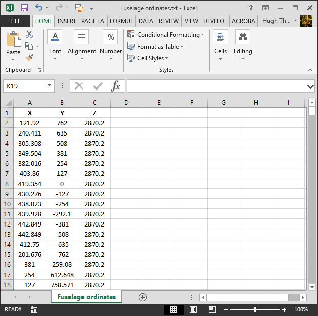
When you start a sketch in Inventor there is a feature on the toolbar to import Excel data. When you import the data there are a few self-explanatory options.

There are of course many ways of doing this and it will vary according to what CAD system you use. Importing all X, Y, Z points in a 3D sketch, for example, will align the ordinates with the current UCS, which in some cases may not be desirable. The Z value is the Frame or Station location relative to the aircraft datum, which essentially translates to being the work plane location. The X, Y values are typically the sketch coordinates normal to the work plane.
If you are working on a 2d sketch and importing the set of points as X, Y, Z values; Inventor will only import the respective X,Y values and ignore the Z value, in fact, it will notify you that it is doing this.
Update: July 2018
The ordinate spreadsheets now have an additional page that compiles the ordinates for each frame with the X,Y,Z components listed separately. This makes it easier to manage the ordinates depending on what CAD system you are importing to.
If you require any further information then please drop me a line.
NAA P-51D & B/C Mustang: Wing Ordinate Major Update:
Thanks to Roland Hallam, I am now in receipt of new verifiable information that has prompted a return to the P51 project and a major update to the wing ordinate data sheets.

Many of the blanks have now been filled in and new additional information added. The above image is a snapshot of the work in progress. The groups highlighted in blue are checked verified dimensions, the red values are those that have changed and those areas remaining in white have prompted an interesting conclusion. Up until now, it was presumed that the wing profiles for the P51D and P51C were the same with the exception of the wing root, however, closer inspection would now suggest that a few rib locations are also slightly different which requires further investigation.
I am still working through the new information and dissecting what is relevant to the P-51D and the P-51B/C variants. This will probably take me a while to evaluate but I am confident that this will result in the most comprehensive dataset yet compiled for the P-51 wings.
I had not expected to return to the P51 project at this time but I’m sure you will agree this is an exciting development.
Technote: Icosahedron Edge Calculation:
Geodesic geometry is rather interesting and occasionally quite challenging. I have recently been involved in a project to explore construction options for a structure based on an Icosahedron form. Although the basic geometry was created using Inventor I was curious about the underlying mathematical formulae pertaining to this type of geometry. I also like to be able to verify key dimensions in the 3d model by separate calculation.
One site I would recommend for calculating this stuff is Rechneronline which provides various options for calculating based on known criteria, an example of which I have shown below.

The formula provided are comprehensive but lacking specifically the formula I was looking for to calculate the edge length for a given radius. The fourth formula in the list does include the value (a) which is the Edge Length and therefore can be transposed to determine the value we need.
Here I have rewritten the fourth formula with the value (a) shown as (L) for clarity.
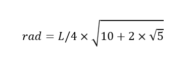
To determine the value (L) the transposed formula would be thus:

This is a small snippet of information that I hope may be of some use for anyone interested in Geodesic geometry. I should note that the 4 is a multiplication of the sum of the parenthesis and not a power to 4 superscript.
To use this in Inventor the formula can be entered as follows in the parameter dialogue box as a user parameter called “EdgeL”:

The resulting Model value verifies the “d112” dimension from the 3d model.


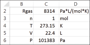
Consider the ideal gas law (Wikipedia) calculation in the Excel spreadsheet in Figure 1.
Contrast the following formulas for calculating the value in cell C6:

Although this is a simple example, the advantage of the formula on the right is evident. In order to reverse-engineer formulas that use cell addresses, such as the one on the left, you would have to trace back the source of each quantity. The formula on the right uses cell names that relate to the variable names from the familiar algebraic ideal gas equation. The style of the spreadsheet layout also improves readability. In Figure 1, the labels in column B are the same as the names for the cells in column C.
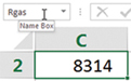
There are three common ways to create names for cells. A convenient method is to select the cell, and type the name into the Name Box field above the column A label:
You can also transfer the label from an adjacent cell onto the cell of interest using Create from Selection in the Defined Names group on the Formula tab of the Ribbon (Figure 2). In fact, more than one label can be transferred with a single command.

▲Figure 2. Create names for cells using the Create from Selection command.
Note that certain names are not allowed. First, you cannot create a name that is the same as a cell address. Given the size of the modern worksheet (the Excel spreadsheet has 214= 16,384 columns and 220 = 1,048,576 rows — a total of 234 cells), with columns out to XFD, it is easy to confuse a name with a cell address. Second, you cannot use the letters R or C as names or those letters followed by any digits. This restriction harkens back to the R-C method of cell addressing (i.e., row-column), which is rarely used today.
The following shows an example of practical formulae using named cells.
It has been said before many times to start at the beginning and finish at the end. For most engineering problems, there is a natural sequence that starts with basic data and proceeds step-by-step to a final result. However, in many calculations, you may need to find one or more starting values that yield a desired final result, or a target value (Figure 3). The target may be a specific value, or it could be the minimum or maximum of a function, such as cost or profitability. The calculation may have more than one input cell, and there may be constraints on various elements of the calculation.
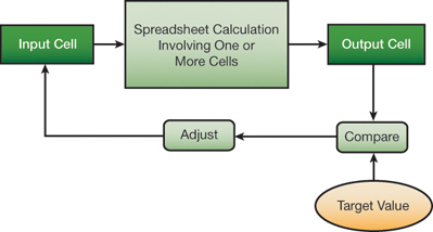
▲Figure 3. Targeting methods, such as Goal Seek or Solver, can help you determine the input value that yields a desired output or target value.
Excel’s Goal Seek is only able to solve target value problems. It is a black-box tool that does not give the user options or control over its numerical procedure. For example, we want to determine the liquid depth in a 4m-diameter spherical tank that corresponds to a volume of 10 m3. The formula is:
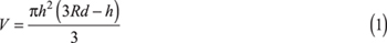
where V is the volume, h is the liquid depth in the tank, and Rd is the radius of the tank. We set up a calculation on the spreadsheet based on a test value of 2 m for the depth (Figure 4a-b).

▲Figure 4. The total volume of a liquid in a tank is calculated for an arbitrary liquid height of 2 m (a) by the formulas shown in (b). Use Goal Seek to set the volume equal to 10 m3 by changing cell h (c) to find the depth corresponding to a 10-m3 volume (d).
Hoppers: Surface Modelling for Mass Containment:
Although not directly associated with aircraft design there are inherent modelling techniques equally applicable to many aspects of aviation. The techniques relate to surface modelling for the containment of a known mass or volume. In each case, the criterion is the specified volume or mass that ultimately defines the size and shape of the container.
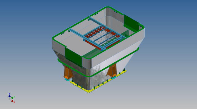
This particular hopper is for a Transfer car used to feed Steel Plant Coke Ovens with coal. The development of this hopper combines surface and solid objects in a single multi-part model that is configurable via a dialogue populated wth the key parameters. Surface modelling can be used for various purposes; some of which I have covered in previous articles for the creation of sheet metal flanges, trimming solids and providing a boundary for extrusion or as a containment for a solid component; as I have used here.

This type of hopper is fed from an overhead bunker and releases the fill material through an aperture in the base. The mass volume is modelled according to industry specifications that define the slope of the poured coal defined by the size of the top bunker opening.
The surface represents the containment boundary which has zero volume and zero mass therefore by definition will ensure that the only properties recorded for mass and volume in the 3d model relate only to the fill material. The image above shows some of the key parameters used to model this hopper as a part file with an ilogic form to make it easier to adjust the parameters to suit the project design.

The gray values for the Coal Volume and the Centre of Gravity are the results calculated from the physical dimensions of the coal mass and the containing surface model. Once the correct dimensional and mass properties are determined the surface objects are extrapolated using the “Make Component” command in Inventor which creates a separate derived part file and also (optional) includes the part file in an assembly placed at the original coordinates. In the surface part file we simply thicken the surface to generate the solid plate material that will form the structural body of the finished hopper.

This is a very basic introduction to using surfaces where the mass or volume of a fill material is the critical component. On some forums, similar questions have been asked for complete hoppers where programmed solutions are offered to subtract all the structural objects to derive the fill mass and volume. By using surfaces with zero mass and volume to contain the fill there is no need for any programming solutions. There are a few ilogic basic routines included in this example for formula calculations and shifting the location of the bunker output. Another example just for reference is the casing for a screwfeeder:

Surfaces are extraordinarily versatile with many applications, only some of which have been mentioned in this blog. For this example, we could extend the technique to modelling fuel tanks, hydraulics and oil tanks where the volume and mass are critical.
